Complexity metrics for 3D meshes • habtools

library(habtools)
library(rgl)
options(rgl.printRglwidget = TRUE)

Checking your mesh

habtools includes a wide range of 3D metrics applicable to meshes.

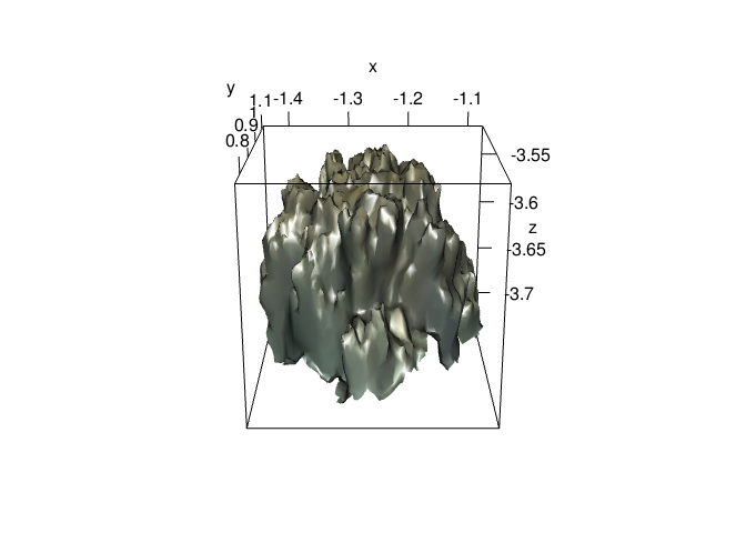
Before calculating any metrics, visualize your mesh and make sure that the z orientation is correct, as this may affect some of the calculations.

plot3d(mcap)

Depending on how the mesh was generated (e.g. with the use of a laser scanner), the resolutions (distance between vertices inside the mesh) can vary a lot. This may affect calculations such as fractal dimension. Check the distribution of resolution of your object and if needed, remesh to make the resolution more uniform.

resvec <- Rvcg::vcgMeshres(mcap)[[2]] # vector of resolutions
hist(resvec)

summary(resvec)
#>     Min.  1st Qu.   Median     Mean  3rd Qu.     Max. 
#> 0.001307 0.005265 0.007003 0.007831 0.009410 0.043981

In our example, the mcap object has very variable distances between vertices. We can solve this issue by re-meshing the object with the Rvcg function vgcUniformRemesh(). Here we set the resolution (voxelSize) to the minimum distance between points in the original mesh to ensure we don’t loose details. This choice may be made on a case-to-case basis. Setting multisample=TRUE improves the accuracy of distance field computation, but slows down the calculation so this choice may be defined by computing power and the size of your object. The re-meshed object now has a mean resolution of approximately the minimum of resvec. While there will still be some variation in the obtained distances between vertices, the variation will be much smaller. An alternative option would be to re-mesh using an external 3D software such as blender.

mcap_uniform <- Rvcg::vcgUniformRemesh(mcap, silent = TRUE, multiSample = TRUE, voxelSize = min(resvec), mergeClost = TRUE)
Rvcg::vcgMeshres(mcap_uniform)[[1]]
#> [1] 0.001328214
summary(Rvcg::vcgMeshres(mcap_uniform)[[2]])
#>      Min.   1st Qu.    Median      Mean   3rd Qu.      Max. 
#> 0.0003464 0.0010450 0.0013561 0.0013282 0.0016327 0.0026663

Complexity metrics: R, D, and H

The three main metrics for DEMs also work for meshes. The recommended method for fractal dimension is cubes.

# fractal dimension
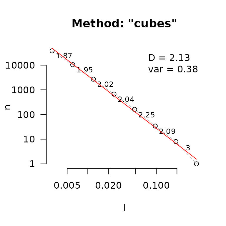
fd(mcap_uniform, method = "cubes", plot = TRUE, diagnose = TRUE)
#> lvec is set to c(0.003, 0.006, 0.012, 0.024, 0.048, 0.096, 0.193, 0.386).

#> $D
#> [1] 2.133279
#> 
#> $data
#>             l     n
#> 8 0.003014892 37982
#> 7 0.006029783 10405
#> 6 0.012059566  2701
#> 5 0.024119132   668
#> 4 0.048238265   162
#> 3 0.096476530    34
#> 2 0.192953059     8
#> 1 0.385906118     1
#> 
#> $lvec
#> [1] 0.385906118 0.192953059 0.096476530 0.048238265 0.024119132 0.012059566
#> [7] 0.006029783 0.003014892
#> 
#> $D_vec
#> [1] 1.868039 1.945711 2.015574 2.043854 2.252387 2.087463 3.000000
#> 
#> $var
#> [1] 0.3837687
#> 
#> $method
#> [1] "cubes"

Rugosity

# rugosity
rg(mcap_uniform)
#> L0 is set to mesh resolution (0.00132821395068341)
#> [1] 3.148722

# height range 
hr(mcap_uniform)
#> [1] 0.2204218

For fractal dimension, two methods are available: cubes and area. In the cubes method, fractal dimension is calculated as the slope of $log10(n) \sim log10(l)$ , where n is the total number of cubes that contains any surface of the object and l is the size of the cubes (elements of lvec). In the area method, the mesh is re-meshed at varying resolutions (lvec). Further, you can calculate planar and total surface area of the object.

planar(mcap)
#> L0 is set to mesh resolution (0.00783124724167033)
#> [1] 0.08303158
surface_area(mcap)
#> [1] 0.2698101

Shape Metrics

There are a number of other metrics that tell you more about the shape of the object. See Zawada et al. (2019) for an example of an application of these metrics on corals.

Convexity: the ratio of the volume of the object and the volume of the convex hull around the object.
Packing: The ratio of the surface area of the object and the surface area of the convex hull around the object.
Sphericity: The ratio of the surface area of a sphere with the same volume as the object and the surface area of the object.
Second moment of area (sma): A measure of top-heaviness using area. Calculated by multiplying the surface area of each triangle in the mesh by its vertical distance from the origin.
Second moment of volume (smv): A measure of top-heaviness using volume. For each triangle in the mesh, a tetrahedron between the triangle and the origin was calculated. The signed volume of each tetrahedron was multiplied by the vertical distance between the centroid of the tetrahedron and the centroid of the attachment plane.
Mechanical shape factor (csf): Mechanical vulnerability of a structural element (Madin & Connolly, 2006).

# convexity
convexity(mcap)
#> [1] 0.4484716

# packing
packing(mcap)
#> [1] 0.8642852

# sphericity
sphericity(mcap)
#> [1] 0.6056971

# second moment of area
sma(mcap)
#> [1] 0.03294466

# second moment of volume
smv(mcap)
#> [1] 0.0005450781

# mechanical shape factor
csf(mcap)
#> z_min set to -3.74007153511047
#> resolution set to 0.00783124724167033
#> [1] 1816.815

Transform mesh into a DEM or 2D shape

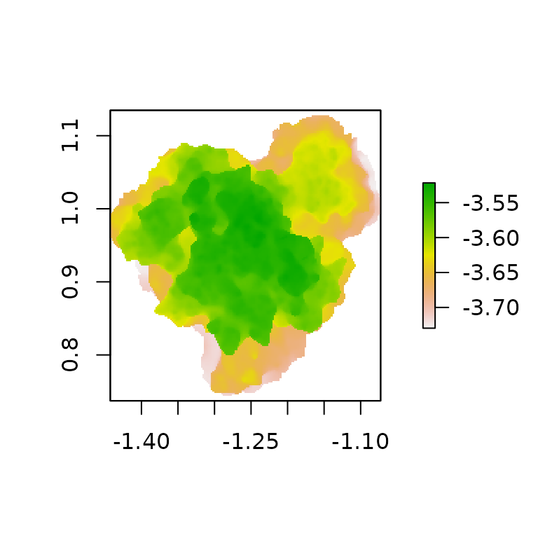
You can also transform a 3D mesh to a DEM, and then apply DEM functions to the surface.

dem <- mesh_to_dem(mcap_uniform, res = 0.002, fill = FALSE)
raster::plot(dem)

rg(dem, method = "area") 
#> [1] 2.767167

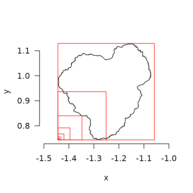
You can also transform a 3D mesh to a 2D drawing, and then apply 2D functions to the object. Note that fractal dimension ranges between 1 and 2 for 2D drawings, rather than 2 and 3 for 3D meshes.

pts <- mesh_to_2d(mcap_uniform)
plot(pts, asp=1)


# perimeter
perimeter(pts)
#> [1] 1.705922

# circularity
circularity(pts)
#> [1] 0.6123799

# fractal dimension
fd(pts, method = "boxes", keep_data = FALSE, plot = TRUE)

#> [1] 1.263879

References

Zawada KJA, Dornelas M, Madin JS (2019) Quantifying coral morphology. Coral Reefs, 38:1281–1292.
Madin JS & Connolly SR (2006) Ecological consequences of major hydrodynamic disturbances on coral reefs. Nature. 444:477-480.